Confidence-based Performance Estimation
Introduction
A binary classification model typically returns two outputs for each prediction - a class (binary) and a class probability predictions (sometimes referred to as score). The score provides information about the confidence of the prediction. A rule of thumb is that, the closer a score is to its lower or upper limit (usually 0 and 1), the higher the probability that a classifier’s prediction is correct. When this score is an actual probability, it can be directly used to calculate the probability of making an error. For instance, imagine a high-performing model which, for a large set of observations, returns a prediction of 1 (positive class) with probability of 0.9. It means that for approximately 90% of these observations, the model is correct while for the other 10% the model is wrong. Assuming properly calibrated probabilities, NannyML reconstructs the whole confusion matrix and calculates ROC AUC for a set of \(n\) predictions according to following algorithm:
Let’s denote:
\(\hat{p} = Pr(y=1)\) - monitored model probability estimate,
\(y\) - target label, \(y\in{\{0,1\}}\),
\(\hat{y}\) - predicted label, \(\hat{y}\in{\{0,1\}}\).
To calculate ROC AUC one needs values of confusion matrix elements (True Positives, False Positives, True Negatives, False Negatives) for a set of all thresholds \(t\). This set is obtained by selecting subset of \(m\) unique values from the set of probability predictions \(\mathbf{\hat{p}}\) and sorting them increasingly. Therefore \(\mathbf{t}=\{\hat{p_1}, \hat{p_2}, ..., \hat{p_m}\}\) and \(\hat{p_1} < \hat{p_2} < ... < \hat{p_m}\) (notice that in some cases \(m=n\)).
The algorithm runs as follows:
Get \(i\)-th threshold from \(\mathbf{t}\), denote \(t_i\).
Get \(j\)-th prediction from \(\mathbf{\hat{p}}\), denote \(p_j\).
Get binary prediction by thresholding probability estimate:
\[\begin{split}\hat{p}_{i,j}=\begin{cases}1,\qquad \hat{p}_j \geq t_i \\ 0,\qquad \hat{p}_j < t_i \end{cases}\end{split}\]
Calculate the estimated probability that the prediction is false:
\[P(\hat{y} \neq y)_{i,j} = |\hat{y}_{i,j} - \hat{p}_{i,j}|\]
Calculate the estimated probability that the prediction is correct:
\[P(\hat{y} = y)_{i,j}=1-P(\hat{y} \neq y)_{i,j}\]
Calculate the confusion matrix elements probability:
\[\begin{split}TP_{i,j}=\begin{cases}P(\hat{y} = y)_{i,j},\qquad y_{i,j}=1 \\ 0,\qquad \qquad \qquad \thinspace y_{i,j}=0 \end{cases}\end{split}\]\[\begin{split}FP_{i,j}=\begin{cases}P(\hat{y} \neq y)_{i,j},\qquad y_{i,j}=1 \\ 0,\qquad \qquad \qquad \thinspace y_{i,j}=0 \end{cases}\end{split}\]\[\begin{split}TN_{i,j}=\begin{cases} 0,\qquad \qquad \qquad \thinspace y_{i,j}=1 \\ P(\hat{y} = y)_{i,j},\qquad y_{i,j}=0\end{cases}\end{split}\]\[\begin{split}FN_{i,j}=\begin{cases} 0,\qquad \qquad \qquad \thinspace y_{i,j}=1 \\ P(\hat{y} \neq y)_{i,j},\qquad y_{i,j}=0\end{cases}\end{split}\]
Calculate steps 2-6 for all predictions in \(\hat{\mathbf{p}}\) (i.e. for all \(j\) from 1 to \(n\)) so that confusion matrix elements are calculated for each prediction.
Get estimated confusion matrix elements for the whole set of predictions, e.g. for True Positives:
\[{TP}_i = \sum_{j}^{n} {TP}_{i,j}\]
Calculate estimated true positive rate and false positive rate:
\[{TPR}_i = \frac{{TP}_i}{{TP}_i + {FN}_i}\]\[{FPR}_i = \frac{{FP}_i}{{FP}_i + {TN}_i}\]
Repeat steps 1-9 to get \(TPR\) and \(FPR\) for all thresholds \(\mathbf{t}\) (i.e. for \(i\) from 1 to \(m\)). As a result, get vectors of decreasing true positive rates and true negative rates, e.g.:
\[\mathbf{TPR} = ({TPR}_1, {TPR}_2, ..., {TPR}_m)\]
Calculate ROC AUC.
Probability calibration
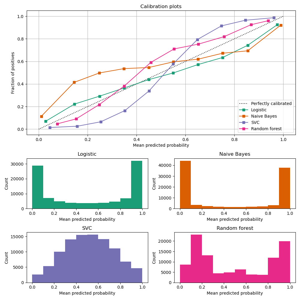
In order to accurately estimate the performance from the model scores, they need to be well calibrated. If a classifier assigns a probability of 0.9 for a set of observations and 90% of these observations belong to the positive class, we consider that classifier to be well calibrated with respect to that subset. Most predictive models focus on performance rather than on probability estimation, therefore their scores are rarely calibrated. Examples of different models and their calibration curves are shown below 1:
Probabilities can be calibrated in post-processing. NannyML uses isotonic regression to calibrate model scores 1 2. Since some of the models are probabilistic and their probabilities are calibrated by design, first NannyML checks whether calibration is required . It is done according to the following logic:
Stratified shuffle split 3 (controlled for the positive class) of reference data into 3 folds.
For each fold, a calibrator is fitted on train and predicts new probabilities for test.
Quality of calibration is evaluated by comparing the Expected Calibration Error (ECE) 4 for the raw and calibrated (predicted) probabilities on the test splits:
If in any of the folds the ECE score is higher after post processing (i.e. calibration curve is worse), the calibration will not be performed.
If in each fold post processing improves the quality of calibration, the calibrator is fitted on the whole reference set and probabilities are calibrated on the set that is subject to analysis.
Calibrating probabilities is yet another reason why NannyML requires reference data that is not a training set of the monitored model. Fitting a calibrator on model training data would introduce bias 1.
References