Confidence-based Performance Estimation (CBPE)
This page describes the algorithms that NannyML uses to estimate post-deployment model performance. At the core of these algorithms NannyML leverages the confidence of the predictions. For classifiers, this confidence is expressed by the probability that an observation belongs to a class. These probabilities are then used to estimate a selected performance metric for a set of observations. Provided that the monitored model returns well-calibrated probabilities (or probabilities that can get well-calibrated in post processing) and a large enough set of observations, CBPE will accurately estimate performance.
CBPE algorithm
Binary classification
A binary classification model typically returns two outputs for each prediction - a class (binary) and a class probability prediction (sometimes referred to as score). The score provides information about the confidence of the prediction. A rule of thumb is that, the closer the score is to its lower or upper limit (usually 0 and 1), the higher the probability that the classifier’s prediction is correct. When this score is an actual probability, it can be directly used to estimate the probability of making an error. For instance, imagine a high-performing model which, for a large set of observations, returns a prediction of 1 (positive class) with a probability of 0.9. It means that for approximately 90% of these observations, the model is correct, while for the other 10% the model is wrong. Assuming properly calibrated probabilities, confusion matrix elements can be estimated and then used to calculate any performance metric. Algorithms for estimating one of the simplest metrics (accuracy) and of the most complex (ROC AUC) are described below. Common notations used in the sections below are the following:
\(n\) - number of analyzed observations/predictions,
\(\hat{p} = Pr(y=1)\) - monitored model probability estimate,
\(y\) - target label, in binary classification \(y\in{\{0,1\}}\),
\(\hat{y}\) - predicted label, in binary classification \(\hat{y}\in{\{0,1\}}\).
Let’s start with accuracy as it should help us to quickly build the intuition. Accuracy is simply the ratio of correct predictions to all predictions. It can be therefore expressed as:
Since the number of observations (\(n\)) is known, the task comes down to estimating True Positives (TP) and True Negatives (TN). The algorithm runs as follows:
Get \(j\)-th prediction from \(\mathbf{\hat{p}}\), denote \(\hat{p}_j\), and predicted label from \(\mathbf{\hat{y}}\), denote \(\hat{y}_j\).
Calculate the estimated probability that the prediction is false:
\[P(\hat{y} \neq y)_{j} = |\hat{y}_{j} - \hat{p}_{j}|\]
Calculate the estimated probability that the prediction is correct:
\[P(\hat{y} = y)_{j}=1-P(\hat{y} \neq y)_{j}\]
Calculate estimated confusion matrix element required for the metric:
\[\begin{split}TP_{j}=\begin{cases}P(\hat{y} = y)_{j},\qquad \ \hat{y}_{j}=1 \\ 0, \qquad \qquad \qquad \hat{y}_{j}=0 \end{cases}\end{split}\]\[\begin{split}TN_{j}=\begin{cases} 0,\qquad \qquad \qquad \hat{y}_{j}=1 \\ P(\hat{y} = y)_{j},\qquad \ \hat{y}_{j}=0\end{cases}\end{split}\]
Get estimated confusion matrix elements for the whole set of predictions, e.g. for True Positives:
\[{TP} = \sum_{j=1}^{n} {TP}_{j}\]
Estimate accuracy:
\[accuracy = \frac{TP+TN}{n}\]
The first three steps are enough to estimate expected accuracy. Once the probabilities of the predictions being correct are known, all that needs to be done is taking the mean of these probabilities. The steps after are there to show how the confusion matrix elements are estimated, which are needed for other confusion-matrix-based metrics like precision, recall etc. Notice, that for models returning a positive class when the probability is larger than 50%, CBPE cannot estimate accuracy lower than 0.5. This is because CBPE works only for models that estimate probabilities well and a model that is worse than a random guess certainly does not do this. Read more in Limitations.
A different type of metric is ROC AUC. To estimate it one needs values of confusion matrix elements (True Positives, False Positives, True Negatives, False Negatives) for a set of all thresholds \(t\). This set is obtained by selecting a subset of \(m\) unique values from the set of probability predictions \(\mathbf{\hat{p}}\) and sorting them increasingly. Therefore \(\mathbf{t}=\{\hat{p_1}, \hat{p_2}, ..., \hat{p_m}\}\) and \(\hat{p_1} < \hat{p_2} < ... < \hat{p_m}\) (\(1 < m \leq n\)).
The algorithm for estimating ROC AUC runs as follows:
Get \(i\)-th threshold from \(\mathbf{t}\) (\(i\) ranges from 1 to \(m\)), denote \(t_i\), .
Get \(j\)-th prediction from \(\mathbf{\hat{p}}\) (\(j\) ranges from 1 to \(n\)), denote \(\hat{p}_j\).
Get the predicted label by thresholding the probability estimate:
\[\begin{split}\hat{y}_{i,j}=\begin{cases}1,\qquad \hat{p}_j \geq t_i \\ 0,\qquad \hat{p}_j < t_i \end{cases}\end{split}\]
Calculate the estimated probability that the prediction is false:
\[P(\hat{y} \neq y)_{i,j} = |\hat{y}_{i,j} - \hat{p}_{j}|\]
Calculate the estimated probability that the prediction is correct:
\[P(\hat{y} = y)_{i,j}=1-P(\hat{y} \neq y)_{i,j}\]
Calculate the confusion matrix elements probability:
\[\begin{split}TP_{i,j}=\begin{cases}P(\hat{y} = y)_{i,j},\qquad \hat{y}_{i,j}=1 \\ 0,\qquad \qquad \qquad \thinspace \hat{y}_{i,j}=0 \end{cases}\end{split}\]\[\begin{split}FP_{i,j}=\begin{cases}P(\hat{y} \neq y)_{i,j},\qquad \hat{y}_{i,j}=1 \\ 0,\qquad \qquad \qquad \thinspace \hat{y}_{i,j}=0 \end{cases}\end{split}\]\[\begin{split}TN_{i,j}=\begin{cases} 0,\qquad \qquad \qquad \thinspace \hat{y}_{i,j}=1 \\ P(\hat{y} = y)_{i,j},\qquad \hat{y}_{i,j}=0\end{cases}\end{split}\]\[\begin{split}FN_{i,j}=\begin{cases} 0,\qquad \qquad \qquad \thinspace \hat{y}_{i,j}=1 \\ P(\hat{y} \neq y)_{i,j},\qquad \hat{y}_{i,j}=0\end{cases}\end{split}\]
Calculate steps 2-6 for all predictions in \(\hat{\mathbf{p}}\) (i.e. for all \(j\) from 1 to \(n\)) so that confusion matrix elements are calculated for each prediction.
Get estimated confusion matrix elements for the whole set of predictions, e.g. for True Positives:
\[{TP}_i = \sum_{j=1}^{n} {TP}_{i,j}\]
Calculate estimated true positive rate and false positive rate:
\[{TPR}_i = \frac{{TP}_i}{{TP}_i + {FN}_i}\]\[{FPR}_i = \frac{{FP}_i}{{FP}_i + {TN}_i}\]
Repeat steps 1-9 to get \(TPR\) and \(FPR\) for all thresholds \(\mathbf{t}\) (i.e. for \(i\) from 1 to \(m\)). As a result, get vectors of decreasing true positive rates and true negative rates, e.g.:
\[\mathbf{TPR} = ({TPR}_1, {TPR}_2, ..., {TPR}_m)\]
Calculate ROC AUC.
Multiclass Classification
A multiclass classification model outputs prediction labels (predicted class) and probabilities for each class. This means that when there are three classes, for example A, B and C, the model output should contain four pieces of information - the predicted class (e.g. A) and three probabilities, one for each class. Assuming these probabilities are well calibrated, they can be used to estimate performance metrics. As an example, let’s describe the process for macro-averaged precision. Let’s use \(c\) to denote total number of classes and \(k\) to indicate a particular class. We can stick to previously introduced notation keeping in mind that \(y\) and \(\hat{y}\) are not binary anymore and take one of \(c\) values.
The algorithm runs as follows:
Estimate precision for each class separately, just like in binary classification. Transform vector of multiclass predictions \(\mathbf{\hat{y}}\) to binary vector relevant for the class \(k\) i.e. \(\mathbf{\hat{y}_k}\) and take corresponding predicted probabilities \(\mathbf{\hat{p}_k}\):
\[{precision}_k = precision(\mathbf{\hat{y}_k}, \mathbf{\hat{p}_k})\]where:
\[\begin{split}\hat{y}_{k,j} = \begin{cases} 1, \qquad \hat{y}_{j}=k \\ 0, \qquad \hat{y}_{j} \neq k\end{cases}\end{split}\]Calculate macro-averaged precision:
\[{precision} = \frac{1}{c} \sum_{k=1}^{c} {precision}_{k}\]
Recall, f1, specificity and one-vs-rest ROC AUC are estimated in the exact same way. Multiclass accuracy is just estimated as the mean of predicted probabilities corresponding to the predicted classes.
Assumptions and Limitations
CBPE is unbiased estimator of performance assuming:
- The monitored model returns well-calibrated probabilities.
Well-calibrated probabilities allow to accurately estimate confusion matrix elements and thus estimate any metric based on them. A model that returns perfectly calibrated probabilities is an ideal probabilistic model (Bayes Classifier). One may ask if there’s anything to estimate if the model is perfect? Performance of an ideal model is usually far from being equal to the maximum possible value for a given metric. It is lower because of the irreducible error originating from classes not being perfectly separable given the available data. In reality, many models are very close to a Bayes Classifier and close enough for CBPE to work. Usually good models (e.g. ROC AUC>0.9) return well-calibrated probabilities, or scores that can be accurately calibrated in postprocessing. There are also models considered as poor (with performance just better than random) that still return well-calibrated probabilities. This happens when dominant share of the error is the irreducible error i.e. when there is not enough signal in the features to predict the target. Performance of all models change in time as a result of changes in the distributions of inputs (X). The good news is that CBPE will remain accurate under data drift i.e. when distribution of inputs P(X) changes but probability of target given inputs P(Y|X) stays the same (or in other words - if probabilities remain well-calibrated). An example might be a situation when one segment of population starts to dominate in the data. In medical applications we might have training data which is balanced with respect to patients’ age but in production mainly older patients are analyzed. Performance of the monitored model will probably change in such case and this change will be noticed by CBPE.
- There is no data drift to previously unseen regions in the input space.
The algorithm will most likely not work if the drift happens to subregions previously unseen in the input space. In such case the monitored model was not able to learn P(Y|X). Using the same example, this will happen when the model was trained on young people only but then it is applied to middle-aged people. If the true relationship between age and the target is nonlinear, most models will not estimate probability correctly on previously unseen data. This also depends on the type of the algorithm used and its ability to extrapolate estimation of probabilities. For example Random Forest model estimated probability will remain constant and equal to the one in the closest input space region covered by training data. In our case this will be the probability for the oldest patients of youngsters. On the other hand, Logistic Regression will learn a parameter (coefficient) between age and the target and then extrapolate linearly. Provided that true underlying relationship is also linear, Logistic Regression model will estimate probability correctly even for unseen age ranges.
- There is no concept drift.
While dealing well with data drift, CBPE will not work under concept drift i.e. when P(Y|X) changes. Except from very specific cases, there is no way to identify concept drift without any ground truth data.
- The sample of data used for estimation is large enough.
CBPE calculates expected values of confusion matrix elements. It means it will get less accurate with decreasing sample size. On top, when the sample size is small it is not just CBPE that won’t work well, but the calculated metric (when targets are available) won’t be reliable either. For example, if we evaluate a random model (true accuracy = 0.5) on a sample of 100 observations, for some samples we can get accuracy as high as 0.65. Read more about it here.
Appendix: Probability calibration
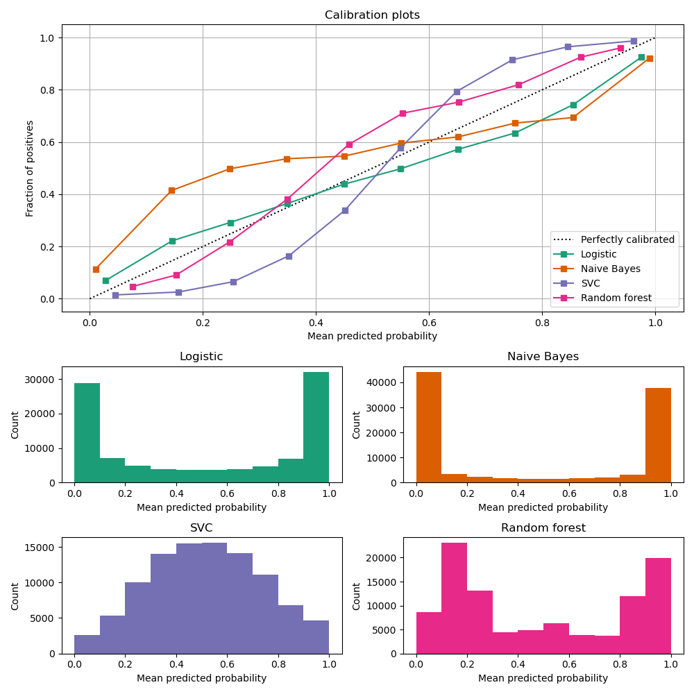
In order to accurately estimate the performance from the model scores, they need to be well calibrated. If a classifier assigns a probability of 0.9 for a set of observations and 90% of these observations belong to the positive class, we consider that classifier to be well calibrated with respect to that subset. Most predictive models focus on performance rather than on probability estimation, therefore their scores are rarely calibrated. Examples of different models and their calibration curves are shown below 1:
Probabilities can be calibrated in post-processing. NannyML uses isotonic regression to calibrate model scores 1 2. Since some of the models are probabilistic and their probabilities are calibrated by design, NannyML will first check if calibration is really required. This is how NannyML does it:
First the reference data gets partitioned using a stratified shuffle split 3 (controlled for the positive class). This partitioning will happen three times, creating three splits
For each split, a calibrator is fitted on the train folds and predicts new probabilities for the test fold.
The Expected Calibration Error (ECE) 4 for each of the test folds is calculated for raw and calibrated probabilities.
The average ECE from all test folds for raw and calibrated probabilities is calculated.
If the mean ECE for calibrated probabilities is lower than the mean ECE for raw probabilities then it is beneficial to calibrate probabilities. Calibrator is fitted on the whole reference set and probabilities get calibrated on the set that is subject to analysis. Otherwise, raw probabilities are used.
For multiclass models the logic above is applied to each class-probability pair separately (so probabilities for some classes might get calibrated while for others not). At the end, probabilities are normalized so they sum up to 1.
Calibrating probabilities is yet another reason why NannyML requires reference data that is not a training set of the monitored model. Fitting a calibrator on model training data would introduce bias 1.
References